Session 2 - Data Literacy: Beyond the Basics

3. Visulising your Data

3.1. Conditional Formatting

Conditional Formatting

Formatted Data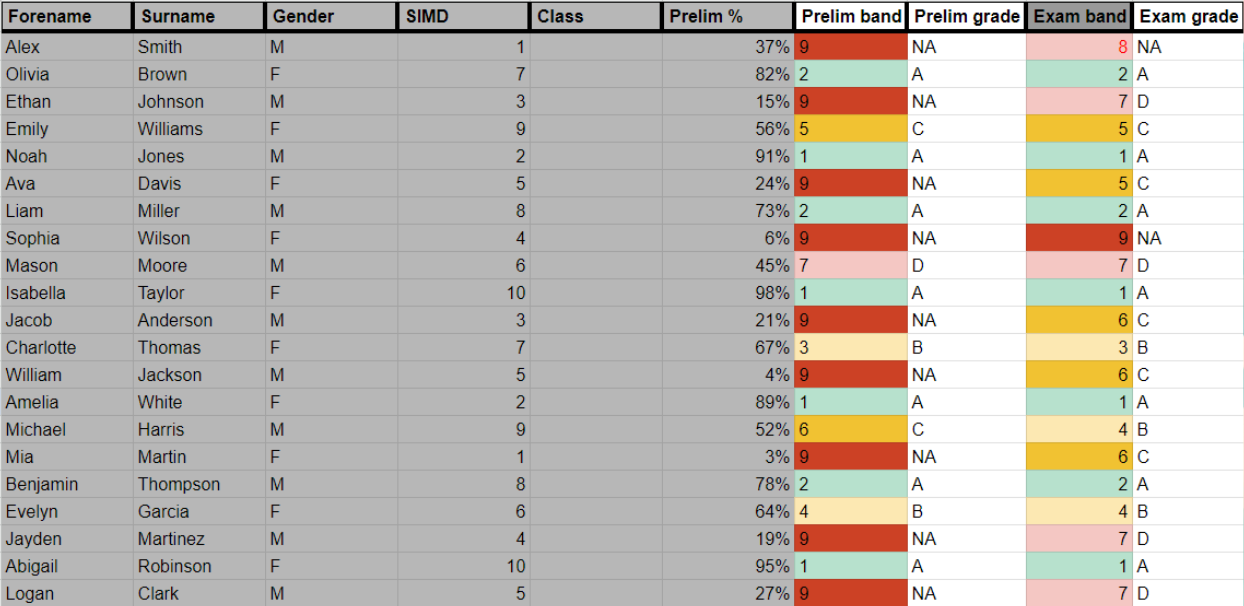

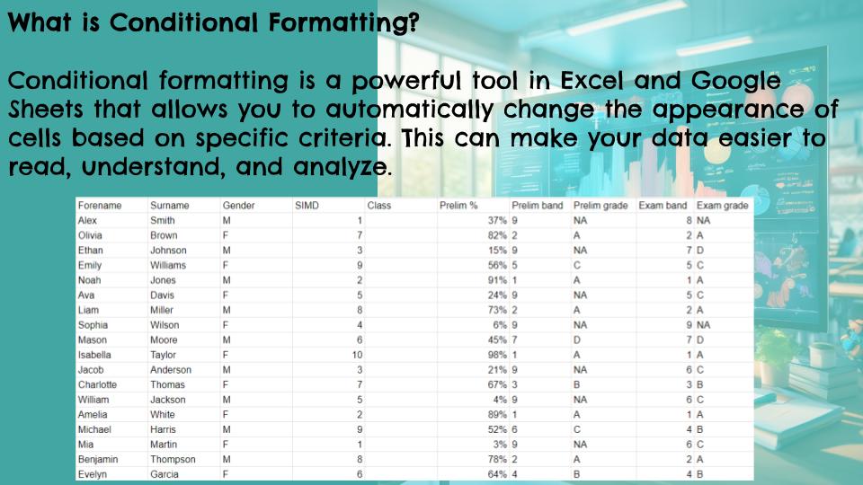
Using Google Sheets: Conditional Formatting

Conditional formatting in Google Sheets lets you automatically apply formatting (like colours, bolding, or italics) to cells based on their values or formulas. This makes it easy to visualize data, highlight important information, and identify trends.

What is Conditional Formatting?

Conditional formatting allows you to set rules that, when met, trigger specific formatting changes in cells. For example, you could highlight all cells containing values greater than 100 in green, or make all dates in the past appear in red.

How to Access Conditional Formatting:

Select the Range: First, select the cells you want to apply conditional formatting to. This can be a single cell, a range of cells, an entire column, or even multiple non-contiguous ranges.
Open the Conditional Format Rules Panel: Go to Format > Conditional formatting in the menu. This will open the Conditional format rules panel on the right side of your sheet.

Applying Conditional Formatting Rules:

The Conditional format rules panel is where you'll define your rules. Here's a breakdown of the key sections:

1. Apply to range:

This shows the selected range where the conditional formatting will be applied. You can adjust the range here if needed.

2. Format rules:

This is where you define the actual formatting rules.

Format rules dropdown: This dropdown offers various pre-built rules, categorized as follows:
- Format cells if...: These rules are based on cell values (e.g., greater than, less than, between, equal to, contains text, date is, etc.).
- Colour scale: These rules create a gradient of colours based on cell values. Useful for visualizing data ranges.
- Data bars: These rules add bars to cells, visually representing the cell values relative to other values in the range.
- Icon sets: These rules add icons to cells, representing the cell values (e.g., arrows, flags, symbols).
- Custom formula is: This option allows you to create complex rules using formulas. This is very powerful for more advanced conditional formatting.
Preview: This shows you a preview of how the formatting will look when the rule is applied.
Formatting style: This section lets you choose the formatting to apply when the rule is met (e.g., background colour, text colour, bold, italics, etc.).

3. Add another rule:

You can add multiple conditional formatting rules to the same range. Rules are evaluated in order, and the first rule that is met will be applied. You can reorder or delete rules as needed.

Example 1: Highlighting Cells Greater Than a Value

Select the range of cells you want to format.
Open the Conditional format rules panel (Format > Conditional formatting).
In the "Format rules" section, choose "Greater than" from the "Format cells if..." dropdown.
Enter the value you want to compare against (e.g., 100).
Choose the formatting you want to apply (e.g., change the background colour to green).
Click "Done".

Example 2: Using a Custom Formula

Let's say you want to highlight rows where the value in column A is greater than the value in column B.

Select the range of cells you want to format (including columns A and B).
Open the Conditional format rules panel.
In the "Format rules" section, choose "Custom formula is" from the "Format cells if..." dropdown.
Enter the following formula: =$A1>$B1 (The `$` before A and B makes the column reference absolute, so it always compares the corresponding values in columns A and B, even if the formatting is applied to other columns.)
Choose the formatting you want to apply.
Click "Done".

Important Considerations:

Rule Order: The order of your conditional formatting rules matters. The first rule that evaluates to TRUE will be applied.
Absolute and Relative References: When using custom formulas, be mindful of absolute ($A$1) and relative (A1) cell references. Absolute references stay fixed when the formatting is applied to other cells, while relative references adjust.
Deleting Rules: You can delete conditional formatting rules from the Conditional format rules panel.

Conditional formatting is a powerful tool for data analysis and visualization in Google Sheets. By mastering these techniques, you can make your spreadsheets more informative and easier to understand.

Using Microsoft Excel: Conditional Formatting

Conditional formatting in Excel allows you to automatically apply formatting (like colours, bolding, or italics) to cells based on their values or formulas. This makes it easy to visualize data, highlight important information, and identify trends.

What is Conditional Formatting?

How to Access Conditional Formatting:

Select the Range: First, select the cells you want to apply conditional formatting to. This can be a single cell, a range of cells, an entire column, or even multiple non-contiguous ranges.
Open the Conditional Formatting Menu: Go to the Home tab on the ribbon, and in the Styles group, click Conditional Formatting. This will open a dropdown menu with various options.

Applying Conditional Formatting Rules:

The Conditional Formatting menu offers various options for creating and managing rules. Here's a breakdown of the key features:

1. Highlight Cells Rules:

This option provides pre-built rules based on cell values (e.g., Greater Than, Less Than, Between, Equal To, Text that Contains, A Date Occurring, Duplicate Values).

2. Top/Bottom Rules:

This option allows you to format the top or bottom N items (e.g., Top 10 Items, Bottom 10%, Above Average, Below Average).

3. Data Bars:

These rules add bars to cells, visually representing the cell values relative to other values in the range.

4. Color Scales:

These rules create a gradient of colours based on cell values. Useful for visualizing data ranges.

5. Icon Sets:

These rules add icons to cells, representing the cell values (e.g., arrows, flags, symbols).

6. New Rule...:

This option opens the "New Formatting Rule" dialogue box, giving you more control over creating custom rules.

7. Clear Rules:

This option lets you clear conditional formatting rules from selected cells or the entire sheet.

8. Manage Rules...:

This option opens the "Conditional Formatting Rules Manager" dialogue box, where you can edit, delete, or change the order of existing rules.

Example 1: Highlighting Cells Greater Than a Value

Select the range of cells you want to format.
Go to Home > Conditional Formatting > Highlight Cells Rules > Greater Than...
Enter the value you want to compare against (e.g., 100).
Choose the formatting you want to apply (e.g., change the fill colour to green) from the dropdown menu or click the "Custom Format..." button for more options.
Click "OK".

Example 2: Using a Formula to Determine Formatting

Let's say you want to highlight rows where the value in column A is greater than the value in column B.

Select the range of cells you want to format (including columns A and B).
Go to Home > Conditional Formatting > New Rule...
Select "Use a formula to determine which cells to format".
Enter the following formula: =$A1>$B1 (The `$` before A and B makes the column reference absolute, so it always compares the corresponding values in columns A and B, even if the formatting is applied to other columns.)
Click the "Format..." button and choose the formatting you want to apply.
Click "OK" twice.

Important Considerations:

Rule Order: The order of your conditional formatting rules matters. The first rule that evaluates to TRUE will be applied. You can manage the rule order in the "Conditional Formatting Rules Manager".
Absolute and Relative References: When using formulas, be mindful of absolute ($A$1) and relative (A1) cell references. Absolute references stay fixed when the formatting is applied to other cells, while relative references adjust.
Clearing Rules: You can clear conditional formatting rules from selected cells or the entire worksheet using the "Clear Rules" option in the Conditional Formatting menu.

Conditional formatting is a powerful tool for data analysis and visualization in Excel. By mastering these techniques, you can make your spreadsheets more informative and easier to understand.

Have a try at some conditional formatting by copying and pasting this demo data into a spreadsheet

Forename	Surname	Gender	SIMD	Class	Prelim %	Prelim band	Prelim grade	Exam band	Exam grade
Alex	Smith	M	1	1A1	37%	9	NA	8	NA
Olivia	Brown	F	7	1A1	82%	2	A	2	A
Ethan	Johnson	M	3	1A1	15%	9	NA	7	D
Emily	Williams	F	9	1A1	56%	5	C	5	C
Noah	Jones	M	2	1A1	91%	1	A	1	A
Ava	Davis	F	5	1A1	24%	9	NA	5	C
Liam	Miller	M	8	1A1	73%	2	A	2	A
Sophia	Wilson	F	4	1A2	6%	9	NA	9	NA
Mason	Moore	M	6	1A2	45%	7	D	7	D
Isabella	Taylor	F	10	1A2	98%	1	A	1	A
Jacob	Anderson	M	3	1A2	21%	9	NA	6	C
Charlotte	Thomas	F	7	1A2	67%	3	B	3	B
William	Jackson	M	5	1A2	4%	9	NA	6	C
Amelia	White	F	2	1A2	89%	1	A	1	A
Michael	Harris	M	9	1A2	52%	6	C	4	B
Mia	Martin	F	1	1A2	3%	9	NA	6	C
Benjamin	Thompson	M	8	1A2	78%	2	A	2	A
Evelyn	Garcia	F	6	1A2	64%	4	B	4	B

Why don't you try:

1. Prelim % (Column E):

Color Scale: Apply a color scale to visually represent the range of percentages. Use a gradient from red (low percentages) to green (high percentages). This provides an immediate visual cue for how well students performed.
Icon Sets: Use icon sets with directional arrows (up, down, sideways) to indicate performance relative to the class average or a target percentage.

2. Prelim Band and Grade (Columns F and G):

Highlight Top Performers: Use a distinct color (e.g., light green) to highlight cells with the highest grade bands (e.g., "1A").
Highlight Students Needing Support: Use a different color (e.g., light red) to highlight cells with the lowest grade bands (e.g., "9N").

3. Exam Band and Grade (Columns I and J):

Improvement/Decline: Use conditional formatting with an icon set to show if a student's performance improved (up arrow), declined (down arrow), or stayed the same (sideways arrow) between the prelim and the exam.
Highlight Significant Changes: Use a rule to highlight cells where the difference between the prelim grade and exam grade is greater than a certain threshold (e.g., 2 grade bands).

4. Gender (Column C):

Differentiation: Use different background colors (e.g., light blue for males, light pink for females) to quickly distinguish between genders. This can help in analyzing performance trends based on gender.

5. SIMD Class (Column D):

Highlight Disparities: Use a color scale to highlight SIMD deciles, with darker shades representing higher deciles. This can help identify any potential correlation between SIMD class and academic performance.